
When studying an algorithm using a direct mapping from a recursive representation of a programme to a recursive representation of a function characterizing its attributes, recurrence relations usually occur. A recurrence is an equation or inequality that reflects the value of a function with smaller inputs. A recurrence can be used to represent the running duration of an algorithm that comprises a recursive call to itself. Time complexities are readily approximated by recurrence relations in many algorithms, specifically divide and conquer algorithms.
Essential Features
The nature of the coefficients involved, the method of combining the terms, and the number and kind of earlier terms used are used to classify recurrences.

Recursion Types with Examples
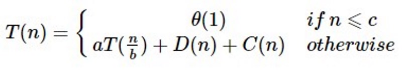
Performing Calculations: In most cases, a recurrence is a quick and easy approach to calculate the amount in question. The first step in approaching any recurrence is to use it to compute tiny numbers to get a sense of how they are expanding. For tiny quantities, this can be done by hand, but for bigger numbers, it’s usually simple to write a programme. Let’s consider an example, where T(n) is the time taken to deal with a problem of size n. The simple solution requires constant time if the task size is small enough, say n<c, where c is a constant and written as θ(1), whereas the time required to find a solution is a.T(n/b) if the problem is broken into n/b sub-problems. If we take the time required for the division to be D(n), and the time required to combine the solutions of sub-problems to be C(n), then, the recurrence relationship can be expressed in the following way:
Recurrence Solution Approaches:
We frequently leave out floors, ceilings, and boundary constraints while stating and solving recurrences. We move forward without this information, deciding afterward whether or not they are important. They typically don’t, but knowing when they do is crucial. Many recurrences encountered in algorithm analysis benefit from the experience, as well as several theorems showing that these aspects have no effect on the asymptotic limits of many recurrences. We’ll go over some of the finer elements of recurrence solution approaches in this section.
The Substitution Approach

The substitution approach entails predicting the answer’s structure, then using mathematical induction to identify the constants and demonstrate that the answer is correct. When the inductive hypothesis is applied to lower numbers, the estimated answer is substituted for the function, thus the name. This approach is effective, but it can only be used in situations when guessing the form of the response is simple. The substitution technique may be used to provide upper and lower boundaries on recurrences. Let’s look at an example of determining a recurrence upper bound.
T(n) = 2T([n/2]) + n
T(n) = O(n lg n) is our best guess for the answer. This approach is used to demonstrate that T(n)≤cn lg n for the proper selection of the constant c > 0. To begin, we assume that this bound holds for [n/2], – i.e., T([n/2])≤c[n/2 ] lg ([n/2]). When you substitute into the recurrence, you get
T(n)≤2(c [n/2] lg ([n/2]))+n
≤cn lg(n/2)+n
=cn lg n-cn lg 2+n
=cn lg n-cn+n
≤cn lg n,
As long as c≥1, the last step is valid. We must now demonstrate that our answer holds for the boundary conditions using mathematical induction – i.e., we must prove that we may select a large enough constant c such that the constraint T(n)≤cn lg n also works for boundary conditions. This need can occasionally cause issues. For the purpose of argument, let’s suppose that T(1) = 1 is the recurrence’s only boundary condition. However, because T(1)≤c1 lg 1 = 0, we won’t be able to pick c big enough.
It is simple to overcome the challenge of establishing an inductive hypothesis given a specified boundary condition. We use the fact that asymptotic notation only compels us to establish T(n)≤cn lg n for n≥n0, where n0 is a constant, to our advantage. The goal is to eliminate the problematic boundary constraint T(1) = 1 from the inductive proof and replace it with n = 2 and n = 3 as part of the proof’s boundary conditions. Because the recurrence does not depend directly on T (1), for n > 3, we may utilise T(2) and T(3) as boundary conditions for the inductive proof . T(2) = 4 and T(3) = 5 are derived from the recurrence. T(n)≤cn lg n for any constant c≥2 may now be completed inductively by choosing c big enough that T(2)≤c2 lg 2 and T(3)≤c3 lg 3. It turns out that any c≥2 will suffice. It’s simple to extend boundary conditions to make the inductive assumption work for small n for most of the recurrences we’ll look at.
The Iteration Approach
It is possible that the method of iterating a recurrence will involve more algebra than the approach of substitution. The goal is to iterate the recurrence such that it may be expressed as a sum of terms that are solely dependent on n and the start conditions. The solution can then be given boundaries using techniques for assessing summations. Consider the occurrence of a recurrence- T(n)=3T([n/4])+n.
This is how we iterate it:
T(n)=n+3T([n/4])
=n+3([n/4]+3T([n/16]))
=n+3([n/4]+3([n/16]+3T([n/64])))
=n+3[n/4]+9[n/16]+27T([n/64]),
where [[n/4]/4] = [n/16] and [[n/16]/4]=[ n/64] from the identity- [[n/a]/b=[n/ab].
How many times must the recurrence be iterated before we hit a boundary condition? 3i [n/4i] is the ith term in the sequence. When [n/4i] = 1 or, equivalently, when I crosses log4 n, the loop reaches n = 1. We learn that the summing comprises a descending geometric series by extending the iteration till this point and applying the constraint [n/4i]≤n/4i:
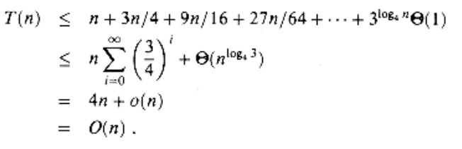
We’ve used the identity alogbn=nlogba to deduce that 3log4 n = nlog43, and we’ve deduced that θ(nlog43) = O(n) using the knowledge that log4 3<1.
The iteration approach normally involves a lot of mathematics, and keeping track of everything may be difficult. The key is to emphasize two parameters: the number of times the recurrence must be iterated in order to meet the boundary condition, and the sum of the terms originating from each iteration level. You can sometimes predict the solution without doing all of the arithmetic when iterating a recurrence. The loop can then be replaced by the substitution approach, which needs less algebra.
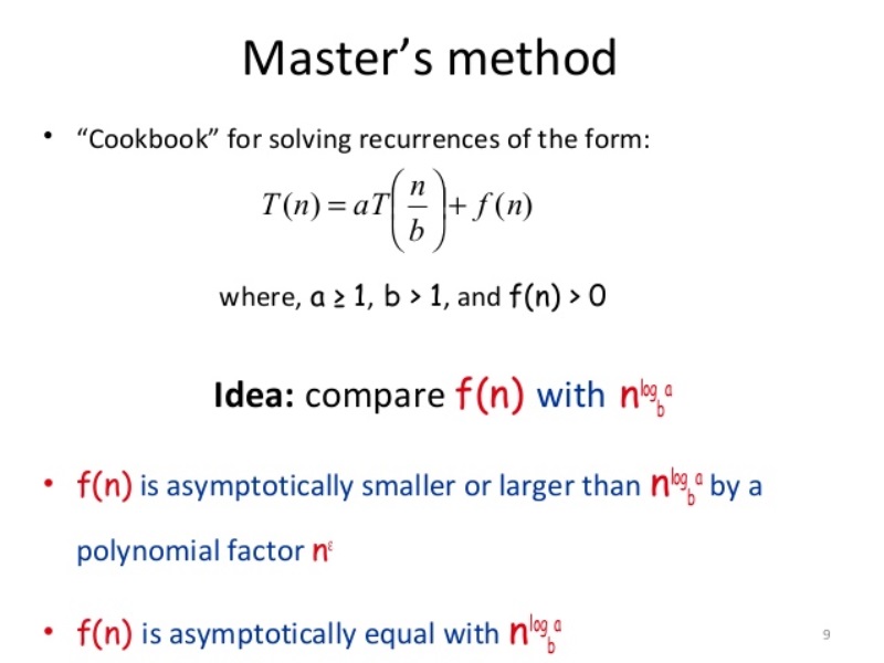
The Master Approach
T(n) = aT(n/b)+â(n),
Where â(n) is an asymptotically positive function, with constants a≥1 and b>1. The master approach necessitates memorizing three cases, but after that, numerous recurrences can be solved quickly, effortlessly, and frequently without the need for pencil and paper. The time it takes for an algorithm to split a problem of size n into ‘a’ sub-problems is described by the recurrence above, where, each sub-problem will be ‘n/b’ in size, with ‘a’ and ‘b’ being positive constants. Each of the ‘a’ sub-problems is solved in time T(n/b) recursively. The function â(n) describes the cost of dividing the task and merging the outcomes of the sub-problems.
The recurrence isn’t properly defined in terms of technical validity because n/b could not be an integer. The asymptotic behavior of the recurrence is unaffected when each of the ‘a’ terms T(n/b) is replaced with either T(n/b) or T(n/b). When creating divide-and-conquer recurrences of this type, it’s usually easier to leave out the floor and ceiling functions.